SYSTEMS DESIGN POWER MANAGEMENT
transformer driver plus a transformer,
two Schottky diodes and an LDO.
Voltage measurement
In order to match the isolated
amplifier’s maximum linear input
voltage range of ±250 mV, Equation
1 calculates the series resistor for
a 100-Ω shunt parallel to the input
pins as:
���������������� = ������������������������ ��������∙√��������∙������������������������ Ω
��������.���������������� �������� = ������������������������. �������� ��������٠(1)
If using one resistor only and it
current and voltage:
burns for whatever reason, this can
create a short to the input voltage
and then the AMC1301 will be
disturbed. Therefore we use several
resistors in series and if one burns
the system stays alive.
Σ ��������������������������������������������������������(��������)�������� ����������������=��������
Σ ��������������������������������������������������������(��������)�������� ����������������
=��������
power = VRMS × IRMS
power = ��������
With the AMC1301’s fixed
voltage gain of 8.2, this results in a
maximum peak-to-peak output voltage
of 2.05 V. Because the integrated
single-ended ADC input range of
the microcontroller is specified with
a voltage range of 0 V to 1.45 V,
the signal needs to be reduced in
amplitude and level shifted.
For optimum performance,
this can be achieved by using the
two operational amplifiers on the
AMC1311 evaluation module. Figure
2 shows the circuit simulated by
TINA-TI software.
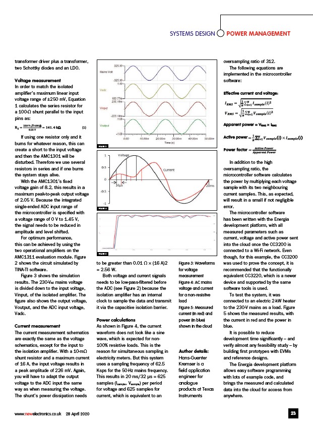
Figure 3 shows the simulation
results. The 230-VAC mains voltage
is divided down to the input voltage,
Vinput, of the isolated amplifier. The
figure also shows the output voltage,
Voutput, and the ADC input voltage,
Vadc.
Current measurement
The current measurement schematics
are exactly the same as the voltage
schematics, except for the input to
the isolation amplifier. With a 10-mΩ
shunt resistor and a maximum current
of 16 A, the input voltage results in
a peak amplitude of 226 mV. Again,
you will have to adapt the output
voltage to the ADC input the same
way as when measuring the voltage.
The shunt’s power dissipation needs
to be greater than 0.01 Ω × (16 A)2
= 2.56 W.
Both voltage and current signals
needs to be low-pass-filtered before
the ADC (see Figure 2) because the
isolation amplifier has an internal
clock to sample the data and transmit
it via the capacitive isolation barrier.
Power calculations
As shown in Figure 4, the current
waveform does not look like a sine
wave, which is expected for non-
100% resistive loads. This is the
reason for simultaneous sampling in
electricity meters. But this system
uses a sampling frequency of 62.5
Ksps for the 50-Hz mains frequency.
This results in 20 ms/32 μs = 625
samples (Isample, Vsample) per period
for voltage and 625 samples for
current, which is equivalent to an
oversampling ratio of 312.
The following equations are
implemented in the microcontroller
software:
Effective and voltage:
Apparent power = VRMS × IRMS
Active power
Power
In addition to the high
oversampling ratio, the
microcontroller software calculates
the power by multiplying each voltage
sample with its two neighbouring
current samples. This, as expected,
will result in a small if not negligible
error.
The microcontroller software
has been written with the Energia
development platform, with all
measured parameters such as
current, voltage and active power sent
into the cloud once the CC3200 is
connected to a Wi-Fi network. Even
though, for this example, the CC3200
was used to prove the concept, it is
recommended that the functionally
equivalent CC3220, which is a newer
device and supported by the same
software tools is used.
To test the system, it was
connected to an electric 2-kW heater
to the 230-V mains as a load. Figure
5 shows the measured results, with
the current in red and the power in
blue.
It is possible to reduce
development time significantly – and
verify almost any feasibility study – by
building first prototypes with EVMs
and reference designs.
The Energia development platform
allows easy software programming
with lots of example code, and
brings the measured and calculated
data into the cloud for access from
anywhere.
Figure 3: Waveforms
for voltage
measurement
Figure 4: AC mains
voltage and current
for a non-resistive
load
Figure 5: Measured
current (in red) and
power (in blue)
shown in the cloud
Author details:
Hans-Guenter
Kremser is a
field application
engineer for
analogue
products at Texas
Instruments
www.newelectronics.co.uk 28 April 2020 23
��������
Σ ��������������������������������������������������������(��������) × ����������������=�������� ��������������������������������������������������������(��������)
= ������������������������������������������������ ����������������������������������������
���������������������������������������������������������� ����������������������������������������
���������������� = ������������������������ ��������∙√��������∙������������������������ Ω
��������.���������������� �������� = ������������������������. �������� ��������
Effective current and voltage:
�������������������������������� = ����������
��������
Σ ��������������������������������������������������������(��������)�������� ����������������=��������
�������������������������������� = ����������
��������
Σ ��������������������������������������������������������(��������)�������� ����������������
=��������
Apparent power = VRMS × IRMS
Active power = ��������
��������
Σ ��������������������������������������������������������(��������) × ����������������=�������� ��������������������������������������������������������(��������)
Power factor = ������������������������������������������������ ����������������������������������������
���������������������������������������������������������� ����������������������������������������
���������������� = ������������������������ ��������∙√��������∙������������������������ Ω
��������.���������������� �������� = ������������������������. �������� ��������
Effective current and voltage:
�������������������������������� = ����������
��������
Σ ��������������������������������������������������������(��������)�������� ����������������=��������
�������������������������������� = ����������
��������
Σ ��������������������������������������������������������(��������)�������� ����������������
=��������
Apparent power = VRMS × IRMS
Active power = ��������
��������
Σ ��������������������������������������������������������(��������) × ����������������=�������� ��������������������������������������������������������(��������)
Power factor
= ������������������������������������������������ ����������������������������������������
���������������������������������������������������������� ����������������������������������������
���������������� = ������������������������ ��������∙√��������∙������������������������ Ω
��������.���������������� �������� = ������������������������. �������� ��������
�������������������������������� = ����������
��������
Σ ��������������������������������������������������������(��������)�������� ����������������=�������� �������������������������������� = ����������
��������
Σ ��������������������������������������������������������(��������)�������� ����������������
=�������� = ��������
��������
Σ ��������������������������������������������������������(��������) × ����������������=�������� ��������������������������������������������������������(��������)= ������������������������������������������������ ����������������������������������������
���������������������������������������������������������� ����������������������������������������FIGURE 3
FIGURE 4
FIGURE 5
/www.newelectronics.co.uk